Cell Anomaly Detection Using Adversarial Autoencoders
Developed an anomaly detection system for cell images using adversarial autoencoders, inspired by the paper "Robust Anomaly Detection in Images using Adversarial Autoencoders" by Laura Beggel, Michael Pfeiffer, and Bernd Bischl.
For detailed documentation and source code, visit my GitHub Repository.
The project focuses on detecting anomalies in images using autoencoder neural networks. An autoencoder learns to reconstruct normal images and can classify images as anomalies when the reconstruction error exceeds a certain threshold. The code in this repository implements an autoencoder-based anomaly detection method using TensorFlow.
Overview

The project addresses a fundamental challenge in anomaly detection using autoencoders, particularly when the training set contains outliers. Continued training of autoencoders tends to raeduce the reconstruction error of outliers, thereby degrading anomaly detection performance. To mitigate this issue, an adversarial autoencoder architecture is employed, which imposes a prior distribution on the latent representation, typically placing anomalies into low likelihood regions. By utilizing the likelihood model, potential anomalies can be identified and rejected during training, resulting in a more robust anomaly detector.
Architecture
The architecture employed in this project leverages a VGG16-based model, modified for the task of encoding and decoding images for anomaly detection. Here’s a breakdown of how the architecture is structured:
-
Encoder: The encoder part of the architecture is based on the VGG16 model, with the fully connected layers removed. The final layer of this modified VGG16 encoder outputs a 7x7x7 encoded image vector. This condensed representation captures the essential features of the input images.
-
Decoder: The decoder mirrors the architecture of the encoder but in reverse. It takes the encoded vector and reconstructs the image. The quality of reconstruction is crucial for detecting anomalies.
#Encoder
model = Sequential()
model.add(Conv2D(64, (3, 3), activation='relu', padding='same', input_shape=(SIZE, SIZE, 3)))
model.add(MaxPooling2D((2, 2), padding='same'))
model.add(Conv2D(32, (3, 3), activation='relu', padding='same'))
model.add(MaxPooling2D((2, 2), padding='same'))
model.add(Conv2D(16, (3, 3), activation='relu', padding='same'))
model.add(MaxPooling2D((2, 2), padding='same'))
#Decoder
model.add(Conv2D(16, (3, 3), activation='relu', padding='same'))
model.add(UpSampling2D((2, 2)))
model.add(Conv2D(32, (3, 3), activation='relu', padding='same'))
model.add(UpSampling2D((2, 2)))
model.add(Conv2D(64, (3, 3), activation='relu', padding='same'))
model.add(UpSampling2D((2, 2)))
- Kernel Density Estimation (KDE): In the middle of the architecture, Kernel Density Estimation (KDE) is used to calculate the likelihood of an image belonging to the ‘good’ class. KDE is applied to the training data to provide an estimate of where the input image vector space lies within the latent space. This estimation helps in determining the ‘normal’ density regions.
- Method: In here build new encoder network, with trained weights from above model.This is used to get the compressed output (latent space) of the input image.The compressed output is then used to calculate the KDE
encoder_model = Sequential()
encoder_model.add(Conv2D(64, (3, 3), activation='relu', padding='same', input_shape=(SIZE, SIZE, 3), weights=model.layers[0].get_weights()) )
encoder_model.add(MaxPooling2D((2, 2), padding='same'))
encoder_model.add(Conv2D(32, (3, 3), activation='relu', padding='same', weights=model.layers[2].get_weights()))
encoder_model.add(MaxPooling2D((2, 2), padding='same'))
encoder_model.add(Conv2D(16, (3, 3), activation='relu', padding='same', weights=model.layers[4].get_weights()))
encoder_model.add(MaxPooling2D((2, 2), padding='same'))
encoder_model.summary()
- Anomaly Detection: Anomalies are determined based on two criteria:
- KDE Value: If the KDE of an image’s latent representation is below a certain threshold, the image is considered an anomaly. This threshold is set based on the density distribution of the training images. Images with latent representations that lie far from the high-density regions (where most training images lie) are flagged as anomalies.
- Reconstruction Error: Additionally, if the reconstruction error (the difference between the original image and its reconstructed image from the decoder) exceeds a predefined threshold, the image is also classified as an anomaly.
This dual-criterion approach helps in robustly identifying images that do not conform to the learned distribution of ‘normal’ images, either through significant deviations in their latent space positioning or through poor reconstruction quality.
def check_anomaly(img_path):
    density_threshold = 2500 #Set this value based on the above exercise
    reconstruction_error_threshold = 0.004 # Set this value based on the above exercise
    img  = Image.open(img_path)
    img = np.array(img.resize((128,128), Image.Resampling.LANCZOS))
    plt.imshow(img)
    img = img / 255.
    img = img[np.newaxis, :,:,:]
    encoded_img = encoder_model.predict([[img]])
    encoded_img = [np.reshape(img, (out_vector_shape)) for img in encoded_img]
    density = kde.score_samples(encoded_img)[0]

    reconstruction = model.predict([[img]])
    reconstruction_error = model.evaluate([reconstruction],[[img]], batch_size = 1)[0]

    if density < density_threshold or reconstruction_error > reconstruction_error_threshold:
        print("The image is an anomaly")

    else:
        print("The image is NOT an anomaly")
Results
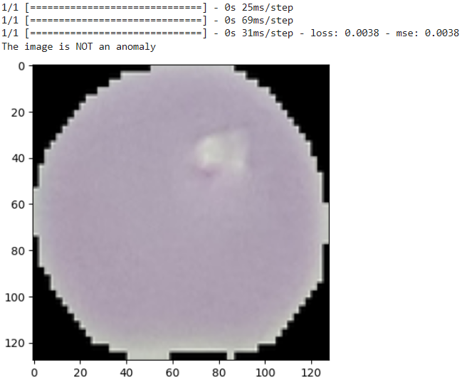
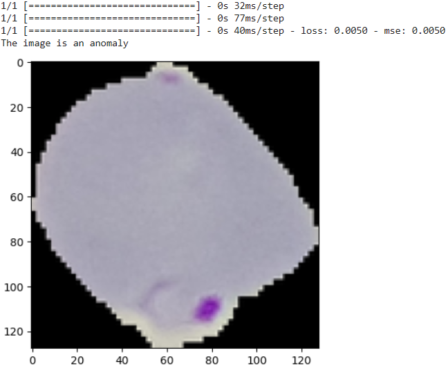
Here below results indicate the model’s effectiveness in recognizing subtle variations in cell morphology associated with anomalies.

